Urban Carbon Cycle
Cities are typical sources of carbon and a focus of climate-change mitigation. Although there is great potential for reducing emissions in cities, constructing low-carbonemission cities under the carbon-emission reduction target of the 2016 Paris Agreement remains challenging as there is little scientific evidence for use by government decisionmakers. To solve this problem, we must understand the urban carbon-cycle process in greater detail and especially analyze spatiotemporal variations in carbon sources and sinks.
1 Carbon sink map
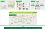
The forest is the only exact carbon sink. How to map the accurate carbon sink maps? Firstly, we propose herein a low-cost method that combines machine learning and spatial statistics to construct a regional biomass map from non-representative sample units. Secondly, we scaled up an ecological process model to obtain the spatial distribution of regional biomass. Finally, we used some data assimilation technology by these data.
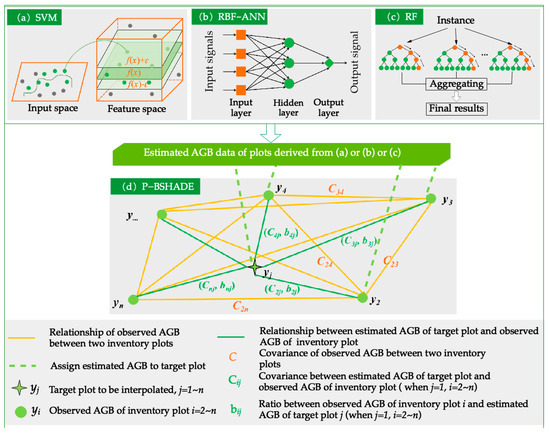
Figure 1 Framework for estimating (a–c) the machine learning models, (d) the P-BSHADE model, and the three models that combine machine learning with the P-BSHADE model ((a,d), (b,d) and (c,d)).
【动态】城市环境研究所在提升森林样地水平地上生物量的估算精度方面取得进展
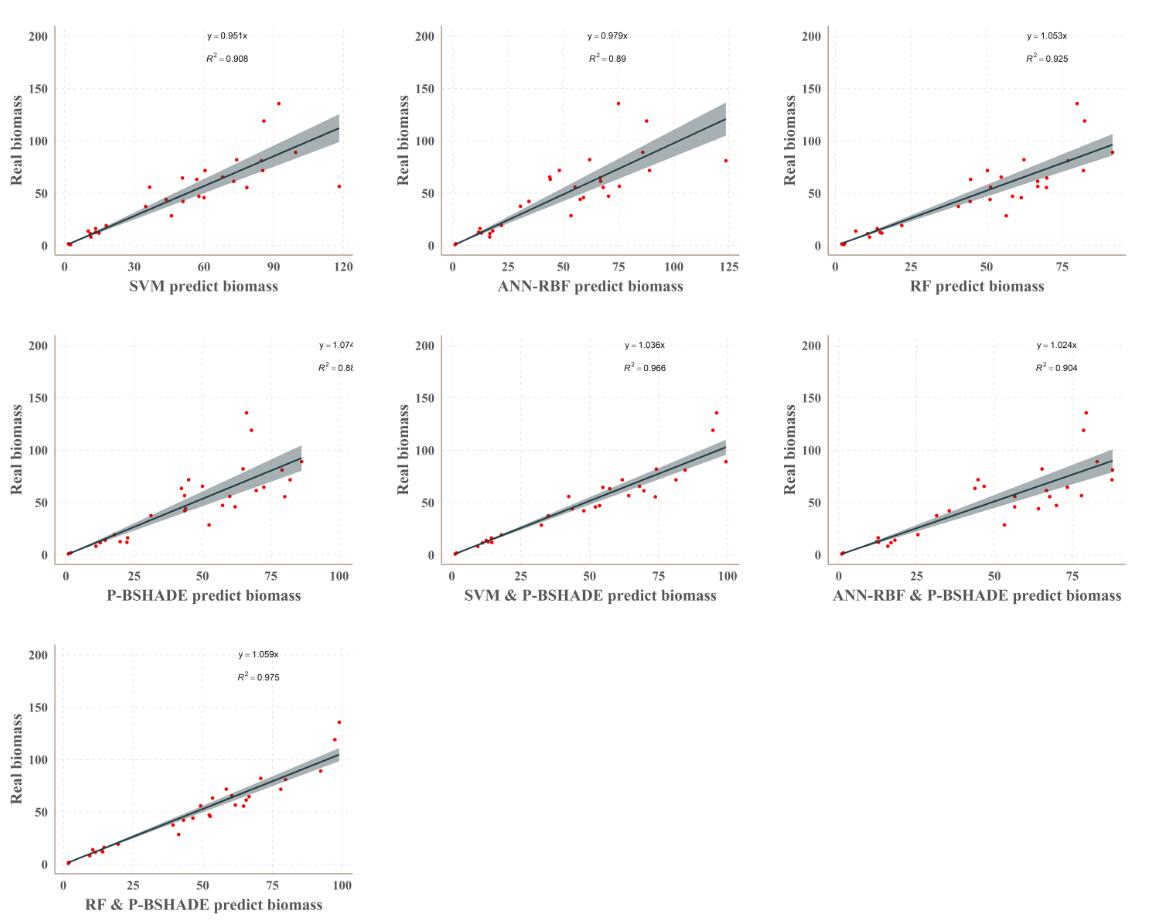
Figure 2. The accuracy of different methods for biomass estimation
2 Carbon source map
Cities are the main sources of $CO_2$ emissions and, thus, must abate emissions responsibly. About 50% of urban $CO_2$ emissions was attributed to urban forms, mixed land use, building types, and transportation networks. It is necessary to characterize the pixel-based distribution of urban direct $CO_2$ emissions accurately. But large uncertainties was found at the urban scale, it’s important to analyze the uncertainties of $CO_2$ emissions gridded map at the urban scale. Besides, exlporing the relationship between $CO_2$ emissions and urban form is useful for planning.
We used a general hybrid approach based on global downscaled and bottom-up elements to produce the CO$_2$ emissions gridded maps, identitfied the urban functional districts map, and generated the city-scale effect related impact factors. All the maps were included in a spatial database. Detailed information can see it.

Figure 3. Comparison between our $CO_2$ emission griddedmap and other inventories
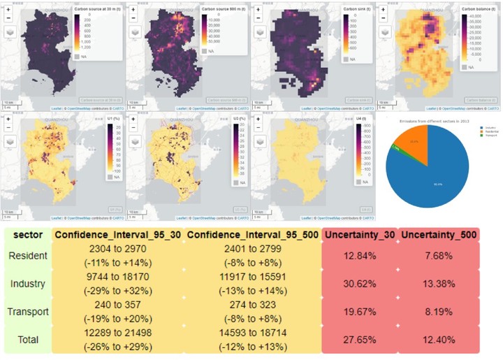
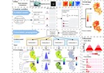
We assessed the uncertainty of CO$_2$ emissions gridded maps during the gridded proceess using our proposed analytic workflow and published in Remote Sensing. Detailed information can see it.
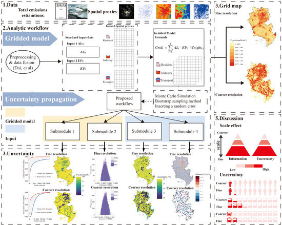
Figure 3. Graphical abstract
Figure 4. The $CO_2$ gridded emissions maps and uncertainty maps
[动态]城市环境研究所在城市尺度二氧化碳排放网格制图的不确定性传播分析取得研究进展
3 The relation between CO$_2$ emissions and urban form
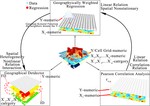
Understanding the spatial or temporal distribution of carbon cycle including carbon sink and source is the key to design low-carbon city development policy. We compared the relationships between urban form fragmentation and CO$_2$ emissions in an urban system through the analytic framework composed of the Pearson correlation analysis, geographically weighted regression (GWR), and geographical detector methods with the use of multi-source data to construct the CO$_2$ emissions maps. The analytical framework can be applied to CO$_2$ emissions research in urban agglomerations, megacities, and small towns.
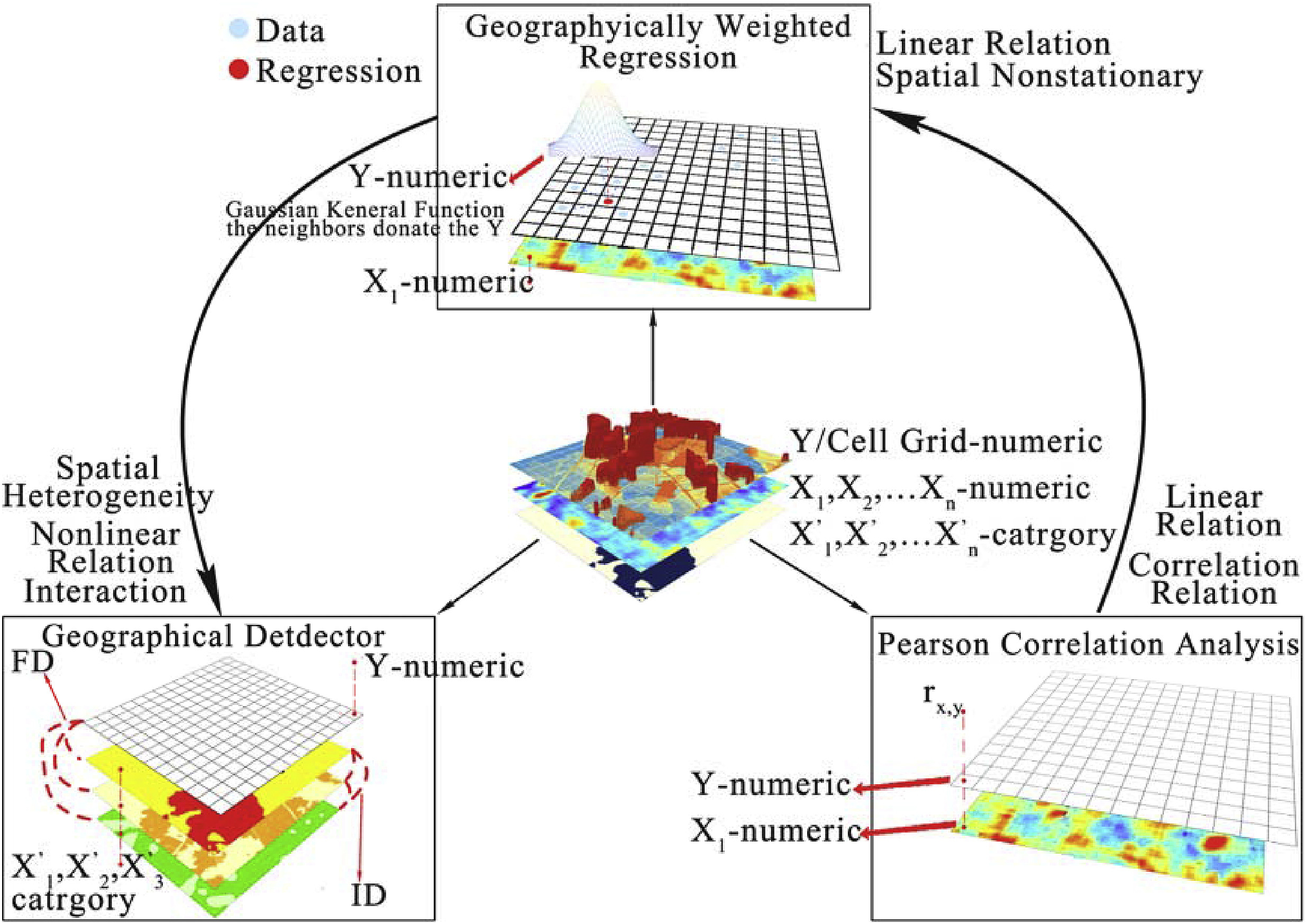
Figure 6. Analytical Framework

Figure 7. Geographical detector results for fragmentation factors, PUA, and POID for CO$_2$ emissions from 4 sources.
This research uses remote sensing data and downscaling interpolation to generate residential and transport (RTCE) maps in 130 m spatial resolution of urban center regions from 31 major cities in China, then investigates the relationship between 3 types of urban form indicators (Internal characteristics, external morphology, and development intensity) and RTCE through Geographical Weighted Regression method. The results reveal that urban form indicators could explain about 45.9% of RTCE. The 2D building shape indicator has the second greatest positive impact as the external morphology indicator, which complicates the influence. The internal characteristics indicators have relatively strong influences than the development intensity indicators. For instance, the influence of functional mixed entropy (FME) is the greatest positive influence and decreases exponentially with FME increases.
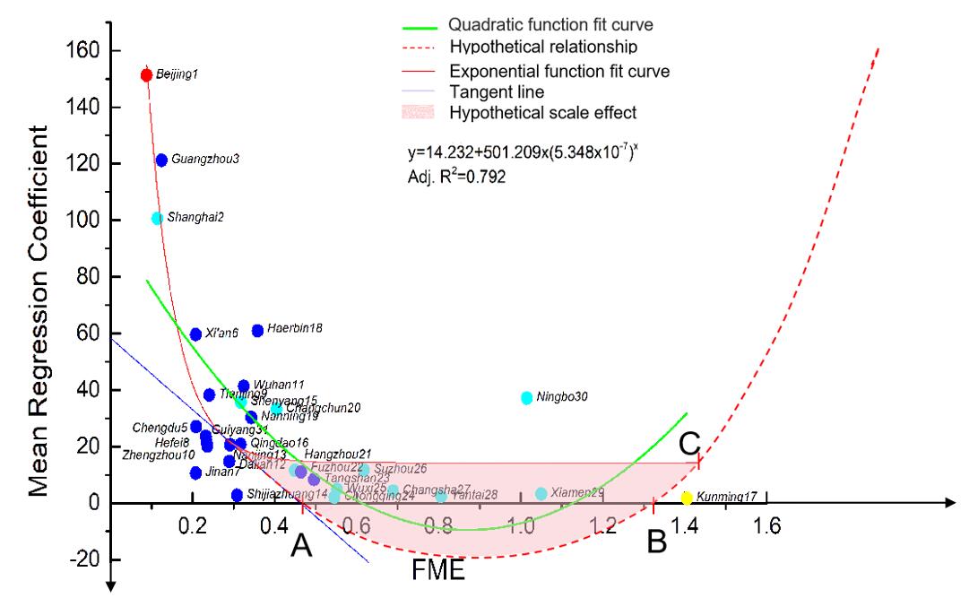
Figure 8. The relation between the functional mixed entropy and the GWR mean regression coefficients in 31 cities. The red, yellow, light blue and blue dot represents the Type Ⅰ, Ⅱ, Ⅲ and Ⅳ city, respectively. The numbers follow the city names represent the size order of the urban area. Point A, B and C are hypothetical.
4 Local carbon emission zone construction
We constructed the local carbon emission zone (LCEZ) which links the highly urbanization morphology profiles and CO$_2$ emission intensity to favor summarizing the form characteristics for the low CO$_2$ emission control in new communities.

Figure 9. The flowchart of the LCEZ construction. Step 1: Luojia1-01 night light image data is the proxy variable of the RTCE map. GWR is geographically weighted regression. Step 2: L is low. M is medium. H is high. the solid line is the three key factors. The dotted line means that n key factors can be selected in the future. The point is POI. the column is BF. the line is RD. A&B represents Dense&sparse forests. C&D represents Farmland&grassland&wetland. G represents the water body.
Shaoqing Dai
Postdoc
Publications
Local carbon emission zone construction in the highly urbanized regions: Application of residential and transport CO$_2$ emissions in Shanghai, China
A predition method of subtropical forest biomass
Improving the accuracy of forest biomass estimate using source analysis and machine learning
A biomass estimation method by fusing plot data and forest inventory data
The importance of the functional mixed entropy for the explanation of residential and transport CO$_2$ emissions in the urban center of China
Improving Plot-Level Model of Forest Biomass: A Combined Approach Using Machine Learning with Spatial Statistics
Investigating the Uncertainties Propagation Analysis of CO$_2$ Emissions Gridded Maps at the Urban Scale: A Case Study of Jinjiang City, China
A spatial database of CO$_2$ emissions, urban form fragmentation and city-scale effect related impact factors for the low carbon urban system in Jinjiang city, China
More fragmentized urban form more CO$_2$ emissions? A comprehensive relationship from the combination analysis across different scales
Creating a Carbon Source and Sink Map by Coupling an Ecological Process Model with an Emission Inventory to Study a Carbon Balance
Improving the prediction accuracy of forest aboveground biomass benchmark map by integrating machine learning and spatial statistics
High-resolution mapping of direct CO$_2$ emissions and uncertainties at the urban scale
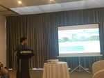
Talks
Application of night light remote sensing data in urban studies
Exploring the impact factors of uncertainties for urban carbon dioxide, a case of Jinjiang, Quanzhou, China
High-Resolution Mapping of Direct CO$_2$ Emissions and Uncertainties at the Urban Scale